Multivariate Regression Analysis

In this project, I explored a  Marketing Dataset that contains information about sales for two consecutive years. Each row contains weekly data about the Volume of Sales and different types of campaign/promotion methods used for the marketing of that product.

I decided to use this data to establish the relationships between Sales Volume and marketing campaigns that were pursued in the course of 2 years. To do so, I will be using Multivariate Regression.

Data at Hand

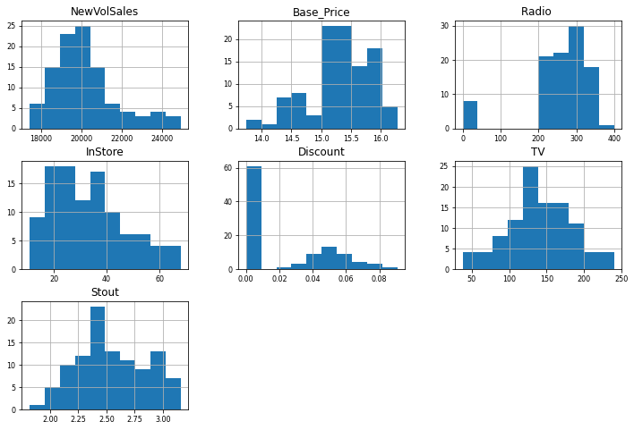
We can see that the dataset is not very large but it is a good amount to demonstrate multivariate regression nicely. Below are the histograms of the rows we are working with:

From these, we can see all of the distributions. In particular, we can see that Discount and Radio have a high frequency at 0. Although this may seem like an outlier, this could be justified by the fact that most items are not discounted and that Radio Promotion was not used frequently. We now need to clean the data and treat the missing values.

Cleaning Data

Here we found that NewVolSales, Base_Price, Radio, InStore, Discount, TV, Stout are the numeric columns so we can drop the columns containing categorical data.

Let's check if we have any n/a values

We see that the only column containing missing values is Radio. We can fill these out with the mean of other values present in the column

Let's look at our data again:

And.. we got rid of all the n/a values. There are no more missing values, and the outliers have been accounted for. This means we can now split this data and train our model.

Multivariate Regression

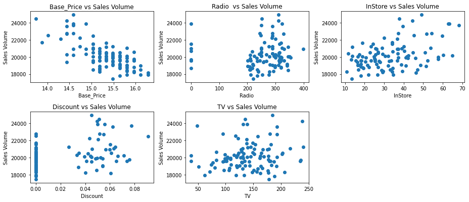
First, we can split this into our X (independent variables) and y (dependent variables). Then we can plot their relationship to the Sales Volume.

Here we see a negative relationship between the Base_Price and the Sales Volume as well as a positive relationship with the InStore column. Now that we have a good idea of the relationship each variable has with the Sales Volume. We can start by splitting the data.

We can check the accuracy of our model looking at R^2

The R^2 value is around 0.66 which is rather low however considering the type of data we are dealing with, it is satisfactory.

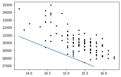
As previously mentioned, there is a strong negative relationship between the Sales Volume and the Base_Price. We can visualise this dimension of the model by plotting a line of best fit.

As we can see here the line of best fit misses the data by a significant amount. This is due to the poor choice of independent variables. In order to remedy this, we should be more rigorous with choosing our independent variables. For example, I suspect that the Discounts variable had a negative impact on the accuracy of this line as it had a lot of values at 0.

Prediction

Nevertheless, this model can still be used for prediction as it follows the correct trend. Below is an example of a prediction made by the model.

Here is the output

We see that for average values of the input parameters we get a prediction order of magnitude.

You can view my Jupyter Notebook using the link below.